cd ~/blogs

May 30, 2026 26 min read 5,111 words

Beyond the Billionth Prime: Pushing Bare-Metal LLVM to the Limit

Bypassing libc, memory bottlenecks, and linear sieves. A deep dive into analytic number theory, Lehmer’s formula, and L3 cache pinning in handwritten LLVM IR.

• #number-theory
• #prime-numbers
• #llvm
• #llvm-ir
• #mathematics
• #lehmer's-algorithm
• #systems-programming
• #bare-metal
• #optimization-algorithms
• #dynamic-programming
• #algorithms
• #performance
• #assembly

---

A few weeks ago I watched SheafificationOfG’s video “One second to find the BILLIONth PRIME”, where he works through a series of increasingly fast prime-finding algorithms — all written in raw, handwritten LLVM IR, no libc — until he can find the billionth prime in under a second. If you haven’t seen it, watch it first. The video is very intuitive and a great watch.

After watching it I couldn’t stop thinking: what’s the actual ceiling here? The final algorithm in the video is Legendre’s formula — already analytic, already sub-linear. But Legendre is the simplest member of a family of progressively more powerful prime-counting methods. Lehmer’s formula, published in 1959, extends Legendre with additional combinatorial terms that dramatically reduce the size of the recursion tree. What if you combined Lehmer with a precise analytic estimate to skip directly to the neighborhood of the target prime, and only sieved a tiny window at the end?

That’s what this experiment is.

The result: given a 1-second timeout, the algorithm finds the 23.76 billionth prime (620,490,072,817) — roughly 85 times further than Legendre’s formula gets in the same time, on the same machine. The performance is very likely to scale with the L3 cache size of the host machine, so I highly encourage you to try it on your own hardware.

This post explains exactly how it works, from the mathematics down to the LLVM IR. There is no hand-waving. Every formula has a corresponding piece of code, and every piece of code has a reason.

The Big Picture: Three Phases

Before diving in, here’s the shape of the entire computation for a large target $n$:

1. Phase 1 — Analytical targeting. Use the inverse of the Logarithmic Integral to predict a number $\hat{x}$ that is close to, but slightly below, the $n$-th prime. This takes microseconds and gets us within a gap of roughly $25\sqrt{\hat{x}}$ of the answer.
2. Phase 2 — Exact count. Use Lehmer’s formula to compute $\pi(\hat{x} - \text{margin})$ — the exact number of primes below the lower edge of our search window — in sub-linear time. This is the heavy part, and the reason the algorithm is fast.
3. Phase 3 — Localized sieve. Run a tiny Sieve of Eratosthenes over the remaining gap, count forward from the exact baseline, and stop when we’ve found the target prime.

If $n \leq 600{,}000$ there’s also a fast path: the startup sieve precomputes (of course dynamically for the sake of the challenge) all primes up to $10^7$, so small queries return instantly from a table. We’ll cover that briefly and move on to the interesting case.

[0x01] The Startup Sieve

Before the main algorithm runs, the program allocates two arrays and populates them with a standard Sieve of Eratosthenes over $[0, 10^7)$:

• pi_table[x] — stores $\pi(x)$, the number of primes $\leq x$, for every $x$ up to $10^7$.
• primes[k] — stores the $k$-th prime (0-indexed, so primes[0] = 2), for the first ~620,000 primes.

The LLVM IR for this lives in src/lehmer/sieve_init.ll. The structure is a textbook Eratosthenes sieve with one detail worth noting: the inner marking loop starts at $p^2$, not $2p$. This is the standard optimization — any composite $m = p \cdot q$ with $q < p$ has already been marked when $q$ was the outer prime. So by the time we process $p$, everything below $p^2$ that’s a multiple of $p$ is already marked.

found_prime:
  %prime.store = getelementptr i64, ptr %primes, i64 %prime_count
  store i64 %p, ptr %prime.store
  %prime_count.inc = add i64 %prime_count, 1
  %p.sqr = mul i64 %p, %p
  br label %mark_loop

mark_loop:
  %mult = phi i64 [ %p.sqr, %found_prime ], [ %mult.next, %mark_step ]
  %mark.done = icmp ugt i64 %mult, %limit
  br i1 %mark.done, label %record_pi, label %mark_step

The pi_table is filled simultaneously: after processing each number $p$ (prime or composite), the current running count of primes found is written to pi_table[p]. By the time the sieve finishes, pi_table[x] holds $\pi(x)$ for all $x \leq 10^7$.

These two arrays become the foundation that every subsequent computation leans on. Any $\pi(x)$ query for $x < 10^7$ is a single array lookup. Any prime $p_k$ for $k < 620{,}000$ is a single array lookup. The rest of the algorithm is built on top of this dynamically precomputed base.

---

[0x02] Finding the Target Neighborhood — The Inverse Logarithmic Integral

The Prime Number Theorem tells us that the number of primes up to $x$ is approximately:

$\pi(x) \sim \text{li}(x) = \int_0^x \frac{dt}{\ln t}$

This approximation is extraordinarily accurate. For $x = 10^{12}$, $\text{li}(x)$ is within about 0.0001% of the true $\pi(x)$. That accuracy is exactly what we need: if we want to find the $n$-th prime, we need an $x$ such that $\pi(x) \approx n$. In other words, we need to invert $\text{li}$.

There’s no closed form for $\text{li}^{-1}(n)$, but we can find it numerically using Newton-Raphson. We want to find the root of:

$f(x) = \text{li}(x) - n = 0$

Newton-Raphson iterates:

$x_{k+1} = x_k - \frac{f(x_k)}{f'(x_k)}$

The derivative of $\text{li}(x)$ is $1/\ln x$ by the fundamental theorem of calculus (since $\text{li}(x) = \int_0^x dt/\ln t$). So:

$x_{k+1} = x_k - \frac{\text{li}(x_k) - n}{1/\ln x_k} = x_k - (\text{li}(x_k) - n) \cdot \ln x_k$

The implementation runs at most 8 iterations of this, with an early exit when the correction step $|(\text{li}(x_k) - n) \cdot \ln x_k|$ drops below 0.5 — meaning the estimate is within half a unit of the true inverse, which is plenty accurate for our purposes.

The initial guess

Before Newton-Raphson starts, we need a starting point $x_0$ that’s already close to the answer. A crude but effective starting estimate comes from inverting the simpler approximation $\pi(x) \approx x / \ln x$:

If $\pi(x) \approx n$, then $x \approx n \ln n$. Using two terms of the asymptotic expansion for $\text{li}^{-1}$:

$x_0 = n \left( \ln n + \ln(\ln n) - 1 + \frac{\ln(\ln n) - 2}{\ln n} \right)$

In the LLVM IR:

define private i64 @inv_li(i64 %n_int) {
entry:
  %n     = uitofp i64 %n_int to double
  %ln_n  = call double @log_fpu(double %n)
  %ln_ln_n = call double @log_fpu(double %ln_n)

  %t1 = fadd double %ln_n, %ln_ln_n      ; ln n + ln ln n
  %t2 = fsub double %t1, 1.0             ; - 1
  %t3 = fsub double %ln_ln_n, 2.0        ; ln ln n - 2
  %t4 = fdiv double %t3, %ln_n           ; / ln n
  %t5 = fadd double %t2, %t4             ; complete correction term
  %x.init = fmul double %n, %t5          ; x_0 = n * (...)

Computing li(x) without a math library

Since there’s no libm, the program computes $\text{li}(x)$ using its asymptotic expansion:

$\text{li}(x) \approx \frac{x}{\ln x} \sum_{k=0}^{14} \frac{k!}{(\ln x)^k}$

This is a divergent asymptotic series, but for large $x$ the first several terms converge rapidly before the factorial growth kicks in. The loop terminates either when the current term drops below $10^{-14}$ in absolute value, or after exactly 14 terms — whichever comes first.

The trick for computing each successive term efficiently: notice that $\frac{k!}{(\ln x)^k} = \frac{(k-1)!}{(\ln x)^{k-1}} \cdot \frac{k}{\ln x}$, so each term is just the previous term multiplied by $k / \ln x$. No factorial computation needed.

define private double @logarithmic_integral(double %x) {
entry:
  %ln_x = tail call double @log_fpu(double %x)
  br label %loop
loop:
  %k      = phi i32    [ 1,   %entry ], [ %k.next,    %latch ]
  %term   = phi double [ 1.0, %entry ], [ %term.next, %latch ]
  %sum    = phi double [ 1.0, %entry ], [ %sum.next,  %latch ]

  %k.f       = uitofp i32 %k to double
  %div       = fdiv double %k.f, %ln_x
  %term.next = fmul double %term, %div     ; term_k = term_{k-1} * k/ln(x)
  %sum.next  = fadd double %sum, %term.next

The sum and term are both initialized to 1.0 before the loop, representing the $k=0$ term $0! / (\ln x)^0 = 1$. The loop then adds terms for $k = 1, 2, \ldots$ The final result is $(x / \ln x) \cdot \text{sum}$.

Computing ln(x) without libm — the fyl2x trick

Every ln call in the program uses a single x87 floating-point instruction: fyl2x. This instruction computes $y \cdot \log_2(x)$. If we pass $y = \ln 2 \approx 0.693147$, we get:

$\ln 2 \cdot \log_2 x = \log_e x = \ln x$

In LLVM IR this is expressed as inline assembly:

define private double @log_fpu(double %x) {
  %fyl2x = call double asm "fyl2x",
    "={st},0,{st(1)},~{st(1)},~{dirflag},~{fpsr},~{flags}"
    (double %x, double 0.6931471805599453)
  ret double %fyl2x
}

The constraint string ={st},0,{st(1)} tells LLVM: the output is the top of the x87 stack (st), the first operand goes into st(0), the second into st(1). ~{st(1)} marks st(1) as clobbered (it’s consumed by fyl2x). One instruction, no software fallback, no libm.

---

[0x03] Counting Primes Exactly — Lehmer’s Formula

After Phase 1 we have an estimate $\hat{x}$ close to the $n$-th prime. Now we need to know exactly how many primes are below some nearby point, so we can figure out how many more we need to count in Phase 3. That exact count comes from Lehmer’s formula.

Lehmer’s formula (1959) is one of the crown jewels of computational number theory. It computes $\pi(x)$ — the exact number of primes up to $x$ — in sub-linear time. Before we can understand the formula itself, we need to understand the function it’s built around.

The partial sieve function φ(x, a)

Define $\phi(x, a)$ as the count of integers in $[1, x]$ that are not divisible by any of the first $a$ primes. So:

• $\phi(x, 0) = x$ (no primes excluded, everything counts)
• $\phi(x, 1) = \lceil x/2 \rceil$ (exclude multiples of 2)
• $\phi(x, 2)$ = integers up to $x$ not divisible by 2 or 3

The key identity is Legendre’s recursion:

$\phi(x, a) = \phi(x, a-1) - \phi\left(\left\lfloor \frac{x}{p_a} \right\rfloor, a-1\right)$

Meaning: start with the count at level $a-1$, then subtract those that are divisible by $p_a$ (since dividing them by $p_a$ leaves a number $\leq x/p_a$ that must not be divisible by $p_1, \ldots, p_{a-1}$).

This recursion is the engine behind both Legendre’s and Lehmer’s formula. The challenge is making it fast, because the recursion tree is enormous.

Lehmer’s formula

Set three limits:

$a = \pi(x^{1/4}), \quad b = \pi(x^{1/2}), \quad c = \pi(x^{1/3})$

Then:

$\pi(x) = \phi(x, a) + \frac{(b+a-2)(b-a+1)}{2} - \sum_{i=a+1}^{b} \pi\left(\frac{x}{p_i}\right) - \sum_{i=a+1}^{c} \sum_{j=i}^{\pi(\sqrt{x/p_i})} \left(\pi\left(\frac{x}{p_i p_j}\right) - (j-1)\right)$

Let’s unpack each term:

• Term 1: $\phi(x, a)$ — the count of integers up to $x$ coprime to the first $a$ primes. Since $p_a = \pi^{-1}(a) \approx x^{1/4}$, any composite number not counted by $\phi(x, a)$ must have all prime factors $\leq x^{1/4}$. The terms that follow correct for the difference between “coprime to the first $a$ primes” and “prime.”
• Term 2: $\frac{(b+a-2)(b-a+1)}{2}$ — a closed-form correction that accounts for primes between $x^{1/4}$ and $x^{1/2}$. These are the primes $p_{a+1}, \ldots, p_b$. The formula is a triangular-number calculation.
• Term 3: $-\sum_{i=a+1}^{b} \pi(x/p_i)$ — subtracts off composites of the form $p_i \cdot q$ where $p_i > x^{1/4}$ and $q \leq x/p_i$. The outer sum runs over primes $p_i$ from just above $x^{1/4}$ to $x^{1/2}$.
• Term 4: the double sum — a fine-grained correction for composites $p_i \cdot p_j \cdot \text{(something)}$ where $p_i, p_j$ are both in a specific range. Each inner term $\pi(x / p_i p_j) - (j-1)$ counts how many primes are paired with $p_i$ and $p_j$ as factors.

This derivation is non-trivial (the original paper is 8 pages of combinatorial argument), but the key practical consequence is that computing $\pi(x)$ this way requires evaluating $\pi$ at many smaller arguments — and those smaller arguments are either in the precomputed table or computable recursively. The recursion depth is bounded, and with memoization the same sub-problems aren’t computed twice.

The LLVM IR implementation

The function lehmer_pi in src/lehmer/lehmer_pi.ll implements this formula. It first checks three caches in order of cheapness:

; 1. Is x within the precomputed pi_table? (free, O(1))
cache_hit:
  %cache.ptr = getelementptr i64, ptr %pi_table, i64 %x
  %cached.val = load i64, ptr %cache.ptr
  ret i64 %cached.val

; 2. Is x in the pi_cache hash table? (near-O(1))
hash_check:
  %hash = mul i64 %x, -7046029254386353131
  %hash_top = lshr i64 %hash, 40         ; extract top 24 bits → 16M-entry table

Only if both caches miss does it actually compute the formula. Once computed, the result is stored back into the hash table for future lookups.

The three roots needed ($x^{1/4}$, $x^{1/2}$, $x^{1/3}$) are computed by integer root functions defined in src/math/roots.ll:

compute:
  %a.input = tail call i64 @iroot4(i64 %x)   ; x^(1/4)
  %a.ptr   = getelementptr i64, ptr %pi_table, i64 %a.input
  %a       = load i64, ptr %a.ptr             ; a = pi(x^(1/4))

  %b.input = tail call i64 @isqrt(i64 %x)    ; x^(1/2)
  %b.ptr   = getelementptr i64, ptr %pi_table, i64 %b.input
  %b       = load i64, ptr %b.ptr             ; b = pi(x^(1/2))

  %c.input = tail call i64 @icbrt(i64 %x)    ; x^(1/3)
  %c.ptr   = getelementptr i64, ptr %pi_table, i64 %c.input
  %c       = load i64, ptr %c.ptr             ; c = pi(x^(1/3))

Term 2 is computed directly:

  %b.plus.a  = add i64 %b, %a
  %term1     = sub i64 %b.plus.a, 2       ; (b + a - 2)
  %b.sub.a   = sub i64 %b, %a
  %term2     = add i64 %b.sub.a, 1        ; (b - a + 1)
  %term.mul  = mul i64 %term1, %term2
  %term.div  = lshr i64 %term.mul, 1      ; divide by 2 via right shift
  %result.init = add i64 %base.phi, %term.div

The outer loop (Term 3 and Term 4) runs from %i = %a to %b - 1 (0-based indexing, so the 0-based %a corresponds to the 1-based $a+1$ in the formula):

loop_i.body:
  %p_i.ptr = getelementptr i64, ptr %primes, i64 %i
  %p_i     = load i64, ptr %p_i.ptr       ; p_{i+1} in 1-based notation
  %w       = udiv i64 %x, %p_i            ; w = floor(x / p_i)

  ; Term 3: subtract pi(x / p_i)
  ; Fast path if w is in precomputed table
  %w_lt = icmp ult i64 %w, %table_limit
  br i1 %w_lt, label %pi_w_fast, label %pi_w_slow

pi_w_fast:
  %pi_w_ptr      = getelementptr i64, ptr %pi_table, i64 %w
  %pi_w_fast_val = load i64, ptr %pi_w_ptr
  br label %pi_w_cont

pi_w_slow:
  %pi_w_slow_val = tail call i64 @lehmer_pi(...)  ; recursive call
  br label %pi_w_cont

For the inner loop (Term 4), notice it only runs when %i < %c (i.e., when $p_i < x^{1/3}$):

  %do_j = icmp ult i64 %i, %c
  br i1 %do_j, label %loop_j.setup, label %loop_i.latch

loop_j.body:
  %p_j.ptr    = getelementptr i64, ptr %primes, i64 %j
  %p_j        = load i64, ptr %p_j.ptr
  %w_div_pj   = udiv i64 %w, %p_j        ; floor(x / p_i / p_j)

  ; This lookup is always in the precomputed table for the scales tested
  %pi_w_pj    = load i64, ptr (getelementptr %pi_table + %w_div_pj)

  %term.sub   = sub i64 %pi_w_pj, %j     ; pi(x/p_i/p_j) - (j-1) in 0-based = pi(...) - j
  %result.j.next = sub i64 %result.j, %term.sub

Note the 0-based index subtlety: the formula subtracts $(j-1)$ in 1-based notation. In 0-based notation, where the loop variable %j corresponds to the 1-based index value $j$, we subtract %j directly — numerically the same value. The README documents this carefully and the code implements it correctly.

Integer roots without libm

The isqrt function uses Newton’s method for integer square roots, with a careful initialisation that guarantees monotone convergence:

define weak_odr i64 @isqrt(i64 %n) {
calc:
  %lz       = tail call i64 @llvm.ctlz.i64(i64 %n, i1 true)
  %active   = sub i64 64, %lz            ; number of significant bits
  %active.plus1 = add i64 %active, 1
  %shift    = lshr i64 %active.plus1, 1  ; ceil(active_bits / 2)
  %guess.init = shl i64 1, %shift        ; initial guess >= true sqrt

loop:
  %guess     = phi i64 [ %guess.init, %calc ], [ %guess.next, %loop ]
  %div       = udiv i64 %n, %guess
  %add       = add i64 %guess, %div
  %guess.next = lshr i64 %add, 1         ; (guess + n/guess) / 2
  %converged = icmp uge i64 %guess.next, %guess
  br i1 %converged, label %return, label %loop

The key insight: by rounding up the initial shift (active_bits + 1 instead of active_bits), the initial guess is always $\geq \sqrt{n}$. Newton’s method then converges monotonically downward, and the loop exits as soon as the next guess is $\geq$ the current one — meaning we’ve hit the floor.

The icbrt function uses binary search instead (Newton’s method for cube roots is less well-behaved numerically at integer precision):

loop:
  %mid   = lshr i64 %diff, 1             ; (high - low) / 2
  %guess = add i64 %low, %mid
  %sq    = mul i64 %guess, %guess
  %cube  = mul i64 %sq, %guess           ; guess^3
  %too_big = icmp ugt i64 %cube, %n
  br i1 %too_big, label %check_high, label %check_low

The search space is bounded at [1, 2097151]. Since $2097151^3 \approx 2^{63}-1$, this safely covers all positive signed 64-bit inputs (and goes vastly beyond our required bounds for the 23-Billionth prime).

---

[0x04] Computing φ(x, a) — The Computational Bottleneck

The most expensive part of Lehmer’s formula is evaluating $\phi(x, a)$. This section explains how the implementation makes it fast enough to be practical.

The naive approach and why it fails

The direct Legendre recursion $\phi(x, a) = \phi(x, a-1) - \phi(\left\lfloor x/p_a \right\rfloor, a-1)$ generates an exponentially large recursion tree. At each node, two sub-problems are spawned. The depth of the tree is $a \approx \pi(x^{1/4})$, which for $x = 10^{12}$ is exactly 168. Without pruning, the tree has $2^{168}$ leaves — completely intractable.

Pruning saves most of it: $\phi(x, a) = x$ when $a = 0$, and $\phi(x, a) = 1$ when $x \leq p_a$ (since only 1 is coprime to all primes up to $p_a$ in that range). But even after pruning, the tree is large. Memoization is the other half of the solution.

The primorial base case: O(1) for a ≤ 6

Instead of recursing all the way down to $a = 0$, the implementation stops at $a = 6$ and uses a precomputed lookup table. Here’s why $a = 6$ is special.

The product of the first 6 primes is:

$p_6^{\#} = 2 \times 3 \times 5 \times 7 \times 11 \times 13 = 30030$

This is called the 6-primorial. The key property: the pattern of which numbers in $[1, 30030]$ are coprime to $\{2, 3, 5, 7, 11, 13\}$ repeats with period exactly 30030. So $\phi(x, 6)$ is periodic modulo 30030:

$\phi(x, 6) = \left\lfloor \frac{x}{30030} \right\rfloor \cdot \phi(30030, 6) + \phi(x \bmod 30030, 6)$

The first term counts how many complete periods fit in $[1, x]$ and multiplies by the count per period. The second term handles the remainder. Both are $O(1)$ once we have the table.

The table precomputed in src/lehmer/phi_init.ll stores $\phi(x, a)$ for all $a \in [0, 6]$ and all $x \in [0, 30030]$. That’s $7 \times 30031 = 210{,}217$ entries of 8 bytes each, totalling $1{,}681{,}736$ bytes — small enough to keep warm in L2 cache.

The initialisation fills row 0 as $\phi(x, 0) = x$, then applies the Legendre sieve step row by row:

inner_loop:
  ; val.prev = phi_table[a-1][n]
  ; val.prev.div = phi_table[a-1][n / p_a]
  ; phi_table[a][n] = val.prev - val.prev.div
  %val.current = sub i64 %val.prev, %val.prev.div
  store i64 %val.current, ptr %ptr.current

This runs once at startup in $O(7 \times 30031) = O(210{,}000)$ time.

The iterative unrolling optimisation

Rather than recursing all the way from depth $a$ down to $a = 6$ one step at a time via the Legendre recursion, the code computes $\phi(x, a)$ in a single iterative sum:

$\phi(x, a) = \phi(x, 6) - \sum_{i=6}^{a-1} \phi\left(\left\lfloor \frac{x}{p_{i+1}} \right\rfloor, i\right)$

This is a telescoping identity derived from the Legendre recursion applied repeatedly. To see why it’s correct: expanding $\phi(x, 7) = \phi(x, 6) - \phi(x/p_7, 6)$, then $\phi(x, 8) = \phi(x, 7) - \phi(x/p_8, 7)$, and continuing, each step adds one term to the sum. By the time we reach depth $a$, we’ve accumulated all the terms in the sum above.

The crucial advantage: each $\phi(\lfloor x/p_{i+1} \rfloor, i)$ call in the sum is itself evaluated using the same function — recursively, but with a smaller first argument and a smaller second argument than the original. The memoization hash table prevents re-computing any $(x', a')$ pair twice.

compute:
  ; Get the O(1) base case
  %base = tail call i64 @phi_eval(i64 %x, i64 6, ...)
  br label %compute_loop

compute_loop:
  %i      = phi i64 [ 6, %compute ], [ %i.next, %compute_loop_step ]
  %result = phi i64 [ %base, %compute ], [ %result.next, %compute_loop_step ]
  %done   = icmp uge i64 %i, %a
  br i1 %done, label %cache_insert, label %compute_loop_step

compute_loop_step:
  %p_i.ptr = getelementptr i64, ptr %primes, i64 %i
  %p_i     = load i64, ptr %p_i.ptr      ; primes[i] = p_{i+1} in 1-based
  %w       = udiv i64 %x, %p_i
  %rec_val = tail call i64 @phi_eval(i64 %w, i64 %i, ...)
  %result.next = sub i64 %result, %rec_val
  %i.next  = add i64 %i, 1
  br label %compute_loop

Memoization with Fibonacci hashing

For any $\phi(x, a)$ call with $a > 6$, the result is cached in a 1 GB open-addressed hash table (64 million 16-byte entries). The hash function uses Knuth’s multiplicative constant:

$\text{hash}(k) = k \times 11400714819323198485 \pmod{2^{64}}$

where the constant is $\lfloor 2^{64} \cdot (\sqrt{5} - 1)/2 \rfloor$ — the golden ratio in 64-bit fixed point. In LLVM IR this is the signed constant -7046029254386353131 (two’s complement representation of the same bit pattern).

The key is packed as key = (x << 16) | a, encoding both arguments into a single 64-bit value. Since $a \leq \pi(x^{1/4})$ grows much slower than $x$, the low 16 bits are always enough for $a$ in practice.

cache_lookup:
  %x_shl = shl i64 %x, 16
  %key   = or i64 %x_shl, %a
  %hash  = mul i64 %key, -7046029254386353131
  %hash_top = lshr i64 %hash, 38    ; extract top 26 bits → 64M entries
  br label %probe_read

probe_read:
  %idx = phi i64 [ %hash_top, %cache_lookup ], [ %idx_next_wrapped, %probe_step ]
  %entry_ptr   = getelementptr { i64, i64 }, ptr %hash_table, i64 %idx
  %stored_key  = load i64, ptr (GEP of key field)
  %is_empty    = icmp eq i64 %stored_key, 0
  br i1 %is_empty, label %compute, label %check_match

probe_step:
  %idx_next         = add i64 %idx, 1
  %idx_next_wrapped = and i64 %idx_next, 67108863   ; mask = 2^26 - 1
  br label %probe_read

Empty slots are detected by stored_key == 0. This works because the key encoding (x << 16) | a is never 0 for any valid $\phi(x, a)$ call that reaches the hash table (both x == 0 and a == 0 return early before the cache is consulted).

The Fibonacci (golden ratio) hash scatters keys uniformly across the table even when inputs are highly structured (e.g., many values of the form $\lfloor C / p_i \rfloor$ which cluster badly under modular hashing). Linear probing on a golden-ratio-hashed table keeps collision chains short in practice.

---

[0x05] The Localized Sieve — Bridging the Final Gap

After Phases 1 and 2, we have:

• $\hat{x}$: our estimate from $\text{li}^{-1}(n)$
• $C = \pi(\hat{x} - \text{margin})$: the exact prime count just below our search window
• $r = n - C$: the number of additional primes to find

Now we just need to find the $r$-th prime at or above $\text{base} = \hat{x} - \text{margin} + 1$. A small Sieve of Eratosthenes handles this.

Sizing the margin

The margin is set to $25\sqrt{\hat{x}}$. Why? By the prime gap theorem, the gap between consecutive primes near $x$ is roughly $\ln x$ on average. Even at $x = 10^{12}$, $\ln x \approx 27.6$. For the logarithmic integral’s error — how far $\text{li}^{-1}(n)$ can be from the true $n$-th prime — the error on the inverse is bounded by $O(\sqrt{p_n} \ln^2 p_n)$ under the Riemann Hypothesis. Setting margin $= 25\sqrt{x}$ gives more than enough room. In practice the overshoot of $\text{li}^{-1}(n)$ over the true $n$-th prime is much smaller than the margin, and the $r$-th prime is always found well within the window.

The sieve spans $[\text{base}, \text{base} + 3 \times \text{margin})$, giving a total of $75\sqrt{\hat{x}}$ bytes to sieve. For $\hat{x} \approx 22.8 \times 10^{9}$ (the scale of the 1-billionth prime) that’s about $75 \times 151{,}000 \approx 11.3$ MB. This is the region that gets sieved; the hot working set during this phase (the sieve array being actively read and written) fits perfectly inside a modern 12 MB L3 cache once the Lehmer computation phase is done.

Marking composites

sieve_primes_loop:
  %p_i = load i64 from primes[i]
  %done = p_i > sqrt(base + gap_size)     ; only need primes up to sqrt(max)
  br if done to scan_gap

mark_gap:
  %rem_div = urem i64 %base, %p_i
  %is_exact = icmp eq i64 %rem_div, 0
  %sub_p    = sub i64 %p_i, %rem_div
  %offset   = select %is_exact, 0, %sub_p  ; first multiple of p_i >= base
  br label %mark_loop

mark_loop:
  %j = phi i64 [ %offset, %mark_gap ], [ %j.next, %mark_step ]
  store i8 1, ptr (gap_sieve + j)          ; mark as composite
  %j.next = add i64 %j, %p_i

For each prime $p_i$ from the precomputed table, the offset of the first multiple of $p_i$ that falls at or above base is computed as:

• If base is exactly divisible by $p_i$, the offset is 0 (i.e., base itself is composite).
• Otherwise the offset is $p_i - (\text{base} \bmod p_i)$, putting us at the next multiple above base.

From that starting point, every $p_i$-th byte is marked as composite. We only need primes up to $\sqrt{\text{base} + \text{gap\_size}}$ — composites with both factors larger than that square root would be larger than the sieve range.

Scanning forward

scan_loop:
  %k         = phi i64 [ 0, %scan_gap ], [ %k.next, %scan_latch ]
  %rem_count = phi i64 [ %rem_target, %scan_gap ], [ %rem.next, %scan_latch ]

  %val      = load i8 from gap_sieve[k]
  %is_prime = icmp eq i8 %val, 0          ; 0 = not marked = prime
  br i1 %is_prime, label %found_prime, label %scan_latch

found_prime:
  %rem.dec   = sub i64 %rem_count, 1
  %is_target = icmp eq i64 %rem.dec, 0
  br i1 %is_target, label %return_ans, label %scan_latch

return_ans:
  %ans   = add i64 %base, %k              ; absolute value of the prime
  %ans_z = zext i64 %ans to i128
  ret i128 %ans_z

The scan walks forward through the sieve one byte at a time, decrementing the remaining count rem_count every time an unmarked (prime) byte is found. When rem_count hits zero, base + k is the $n$-th prime.

The return type is i128 — 128-bit integer — even though all current inputs fit in 64 bits. This is a design choice for forward compatibility: the pipeline is intrinsically capable of returning primes beyond the 64-bit range once the hash table and sieve allocation limits are extended.

---

[0x06] The Bare-Metal Layer

None of the above uses any standard library. Every interaction with the OS is a raw syscall.

Entry point: _start, not main

Standard C programs have main called by the C runtime (crt0), which sets up the environment, processes atexit handlers, and so on. This program defines _start instead — the actual entry point the Linux kernel jumps to when it loads the executable.

define void @_start() naked {
  tail call void asm sideeffect "", "{rbp}"(i64 0)   ; clear frame pointer

  ; On program entry, the stack layout is:
  ;   rsp+0:  argc
  ;   rsp+8:  argv[0]
  ;   rsp+16: argv[1]  <-- our N argument
  %rsp  = tail call ptr asm "", "={rsp},0"(ptr undef)
  %argc = load i64, ptr %rsp
  %argv = getelementptr i8, ptr %rsp, i64 8

  %exitcode = tail call i64 @main(i64 %argc, ptr %argv)
  tail call void @exit(i64 %exitcode)
  unreachable
}

The naked attribute suppresses LLVM’s automatic stack frame setup. The inline assembly reads %rsp directly to get the kernel-populated argc/argv values. When the computation finishes, exit issues syscall 60 (sys_exit) directly, skipping all atexit handlers.

Memory allocation: mmap, not malloc

All heap allocation uses mmap with MAP_PRIVATE | MAP_ANONYMOUS (flags 0x22 = 34):

%pi_table  = call ptr @mmap(ptr null, i64 80000000, i64 3, i64 34, i64 -1, i64 0)
%primes    = call ptr @mmap(ptr null, i64 80000000, i64 3, i64 34, i64 -1, i64 0)
%phi_table = call ptr @mmap(ptr null, i64 1681736,  i64 3, i64 34, i64 -1, i64 0)
%hash_table = call ptr @mmap(ptr null, i64 1073741824, i64 3, i64 34, i64 -1, i64 0)
%pi_cache  = call ptr @mmap(ptr null, i64 268435456,  i64 3, i64 34, i64 -1, i64 0)

PROT_READ | PROT_WRITE = 3. Anonymous mappings are zero-initialised by the kernel — which is precisely what the hash tables rely on (the zero sentinel for empty slots). malloc adds an unnecessary layer; mmap gives us exactly what we need directly.

---

Putting It All Together

For a concrete example, let’s trace what happens when you run ./fast-primes 1_000_000_000:

1. The input is parsed (underscores ignored) to $n = 1{,}000{,}000{,}000$. Since $n > 600{,}000$, we skip the fast path.
2. Phase 1: inv_li(1_000_000_000) runs Newton-Raphson starting from $x_0 \approx 10^9 \cdot (\ln(10^9) + \ln(\ln(10^9)) - 1 + \ldots)$ and converges to $\hat{x} \approx 22{,}801{,}900{,}000$ within 8 iterations.
3. Margin: $\text{margin} = 25\sqrt{22{,}801{,}900{,}000} \approx 25 \times 151{,}004 \approx 3{,}775{,}100$. So $\text{base} = \hat{x} - \text{margin} + 1 \approx 22{,}798{,}124{,}901$.
4. Phase 2: lehmer_pi(base - 1) computes $\pi(22{,}798{,}124{,}900)$ using Lehmer’s formula. This recursively decomposes into calls to phi_eval, isqrt, icbrt, iroot4, and many sub-calls to lehmer_pi — all memoized. The result is some $C$, and the remaining target is $r = 10^9 - C$.
5. Phase 3: A byte sieve of $3 \times 3{,}775{,}100 \approx 11.3$ MB is allocated and marked using primes up to $\sqrt{22{,}798{,}124{,}900 + 11{,}325{,}300} \approx 151{,}028$. The scan walks forward, counting primes until $r = 0$.
6. The answer — 22,801,763,489 — is printed to stdout as 22_801_763_489.

The whole thing runs in roughly 75ms on an i5-12450H. The same machine, running Legendre’s formula from the video, reaches only the ~279 millionth prime in one second. The deeper recursion pruning in Lehmer, combined with the precise analytic targeting, accounts for the ~85× gap.

---

[0x07] What Legendre’s Formula Was Actually Doing — and Why Lehmer Goes Further

The algorithm that concluded the video — Legendre’s formula as implemented in SheafificationOfG/QueenJewels — is already analytic. It doesn’t scan from 2 to $p_n$. It uses a combinatorial formula to count primes sub-linearly, combined with a segmented sieve to collect the small prime base it needs. Understanding exactly what it does, and precisely where it runs out of headroom, is the clearest way to see why Lehmer gains another ~85× on top of it in the same second.

The core idea: Legendre’s formula with a wheel sieve

The QueenJewels prime function follows a two-stage structure:

• Stage 1 — Build a prime base. A segmented sieve populates an array of PrimeInfo structs (prime value + wheel index) for all primes up to approximately $\sqrt{x_{\text{max}}}$, where $x_{\text{max}}$ is a rough upper bound computed for the target $n$. This array is the sieve’s “small primes” reference, used to mark off composites in all subsequent segments.
• Stage 2 — Fast-forward then scan. Rather than sieving from 2 all the way to the answer, the algorithm uses Legendre’s formula via its internal pi function to skip ahead to a segment starting near the answer, then scans forward segment-by-segment until it finds the $n$-th prime.

The wheel factorisation is the main distinguishing feature. Instead of stepping through every integer (including obviously composite ones like even numbers), the sieve maintains a wheel — a compact cyclic list of offsets that skips over all multiples of the first several primes by construction. For a wheel built on the first 5 primes ($\{2, 3, 5, 7, 11\}$, period $2310$), only integers coprime to $2310$ are ever visited. This dramatically reduces the work per segment:

define private %WheelInfo @wheel.extend(...) {
  ; new period = old period * p_new
  %new.period = mul i64 %wheel.period, %prime
  ; new size = old size * (p_new - 1)
  ; (Euler's totient: multiplying by (p-1)/p times old period)
  %new.size   = mul i64 %wheel.size, %prime.m1

The wheel.extend function builds the new wheel by generating all integers in the new period that are coprime to all primes in the wheel, explicitly skipping those that would be eliminated by the new prime. The delta array stores the gaps between successive wheel elements, so the inner mark loop can step through the sieve in variable-sized jumps rather than uniform strides, never landing on a number the wheel already ruled out.

The phi.compute shortcut

The QueenJewels implementation includes a noteworthy optimisation inside its $\phi$ recursion: the shortcircuit block. When a recursive call returns 1 — meaning only one integer in the range is coprime to all primes in the set — the algorithm knows that all remaining terms in the sum will also return 1. Instead of making those calls explicitly, it counts them directly:

shortcircuit:
  ; When phi(x/p_k, k) == 1, every subsequent phi(x/p_l, l) for l > k
  ; where p_l <= x is also 1. Count them by scanning forward.
sc.continue:
  %l.scan = add i64 %l.prev, 1
  %sc.tally = sub i64 %sc.tally.prev, 1  ; subtract 1 for each such term
  %p.l = call i64 @load_prime(..., i64 %l.scan)
  %p.l.small = icmp ule i64 %p.l, %x
  br i1 %p.l.small, label %shortcircuit, label %sc.finish

This is a real pruning improvement. But it’s bounded: it only activates at the leaves of the recursion tree where values have become very small. The tree itself still has to be traversed to get there.

The lower_bound fast-forward and its integer truncation

The lower_bound function computes which segment to jump to before scanning:

define private i64 @lower_bound(i64 %n, i64 %segm.size) {
  %n.p1.trunc = trunc i64 %n.p1 to i32   ; lower bound will be way off if %n is really big :)
  %n.p1.f32   = sitofp i32 %n.p1.trunc to float
  %log.n      = call fast float @log(float %n.p1.f32)

Note the comment in the source — “lower bound will be way off if %n is really big.” It is actually much worse than that. The truncation to i32 acts as a modulo $2^{32}$ operation ($4,294,967,296$). This means any $n \geq 2^{32}$ completely loses its upper bits and silently wraps around.

Because the code uses sitofp (Signed Integer to Float), the behavior fractures into two catastrophic failure modes depending on where those truncated bits land:

1. The Massive Undershoot: If the truncated 32 bits form a positive signed integer (e.g., $n = 5$ Billion truncates to $705$ Million), the log math “succeeds”. But it calculates a boundary for a fraction of the actual target, dropping the program billions of numbers short and forcing the linear sieve to run until the timeout kills it.
2. The NaN Bomb: If the truncated 32 bits form a negative signed integer, the math shatters. For our $n = 23,762,554,725$ target, the truncation yields 2,287,718,246, which is -2,007,249,050 in signed two’s complement. The FPU attempts to calculate log(negative_number), throws a Domain Error, and yields NaN.

For the 23-billion range, the QueenJewels fast-forward math literally disintegrates.

The fundamental asymptotic difference

Both Legendre and Lehmer are analytic prime-counting formulas — neither scans through integers linearly. The difference is in how aggressively they prune the $\phi(x, a)$ recursion tree.

Legendre’s formula is:

$\pi(x) = \phi(x, a) + a - 1$

where $a = \pi(\sqrt{x})$. This requires evaluating $\phi(x, a)$ with $a \approx \pi(x^{1/2})$, meaning the recursion runs to depth $\approx x^{1/2} / \ln x$. The standard complexity for Legendre’s method is roughly $O(x / \log^2 x)$ depending on the caching strategy — sub-linear, but severely bottlenecked by the tree size.

Lehmer’s formula adds two extra correction terms involving $\pi(x^{1/3})$ and $\pi(x^{1/4})$. This sounds like more work, but the additional terms allow the recursion depth to be cut to $a = \pi(x^{1/4})$ instead of $\pi(x^{1/2})$. That shallower depth is the entire game: the recursion depth exponent drops from $1/2$ to $1/4$, which dramatically shrinks the set of distinct $(x', a')$ sub-states that memoization must cover. With memoization, the practical cost of the Lehmer $\phi$ evaluation is $O\left(x^{2/3}\right)$ — substantially better than Legendre’s $O\left(x / \log^4 x\right)$ at large $x$.

By the prime number theorem, $p_n \approx n \ln n$, so at $x = p_n$:

• Legendre: cost $\approx O\left(\frac{n \ln n}{\log^2(n \ln n)}\right) \approx O\left(\frac{n}{\log n}\right)$
• Lehmer (memoized): cost $\approx O\left((n \ln n)^{2/3}\right)$

For $n = 10^9$: Legendre is roughly $10^9 / 20.7 \approx 4.8 \times 10^7$, while Lehmer is roughly $(10^9 \times 20.7)^{2/3} \approx 7.5 \times 10^6$ — roughly a 6.4× gap in raw theoretical $\phi$ operation count. But this understates the real-world advantage, because the QueenJewels implementation also pays the cost of the scanning phase for any $n$ its lower_bound estimate misses (see below), whereas fast-primes always scans only a mathematically bounded $\approx 75\sqrt{p_n}$-byte window regardless of $n$.

At scale, this theoretical difference is massive. While Legendre’s combinatorial tree limits its practical reach to the low hundreds of millions within a second, Lehmer’s $O((n \ln n)^{2/3})$ scaling allows it to push effortlessly into the tens of billions. But even this understates the real-world advantage: because the QueenJewels implementation relies on a conservative lower_bound estimate, it often pays a massive linear scanning cost to bridge the gap to the answer, whereas fast-primes always scans a mathematically bounded $\approx 75\sqrt{p_n}$-byte window regardless of $n$.

A concrete comparison: what each algorithm does for n = 1,000,000,000

Step	QueenJewels (Legendre)	fast-primes (Lehmer)
Estimate target location	lower_bound: $x \approx n \ln n$ via 32-bit float	inv_li: Newton-Raphson on $\text{li}^{-1}(n)$, 8 iterations, double precision
Build prime base	Sieve all primes up to $\sqrt{x_{\text{max}}}$ (~151,000 primes), storing wheel indices	Sieve all primes up to $10^7$ (~620,000 primes), storing values and $\pi(x)$ for $x \leq 10^7$
Count primes to baseline	Legendre’s pi called to count primes below the fast-forward point	Lehmer’s formula called once on $\hat{x} - \text{margin}$, exact count returned
Scan to answer	Sieve consecutive 32KB segments ($\approx 262{,}144$ bits each) forward from the fast-forward point until the $n$-th prime is found	Byte-sieve of $3 \times \text{margin} \approx 11$ MB, scanned once linearly
$\phi$ recursion depth	$a = \pi(x^{1/2})$ — deeper tree, harder to memoize effectively	$a = \pi(x^{1/4})$ — shallower tree, memoization far more effective

The scanning phase difference is the one that shows up most viscerally in benchmarks. Legendre’s lower_bound is deliberately conservative — it undershoots so it never misses the answer — which means the scanning phase has to cover a larger gap. Lehmer’s formula, called once on a precisely targeted $\hat{x} - \text{margin}$, returns an exact count, and Phase 3 scans only the $\approx 11$ MB window between that baseline and the answer.

Algorithmic Performance Scaling Comparison

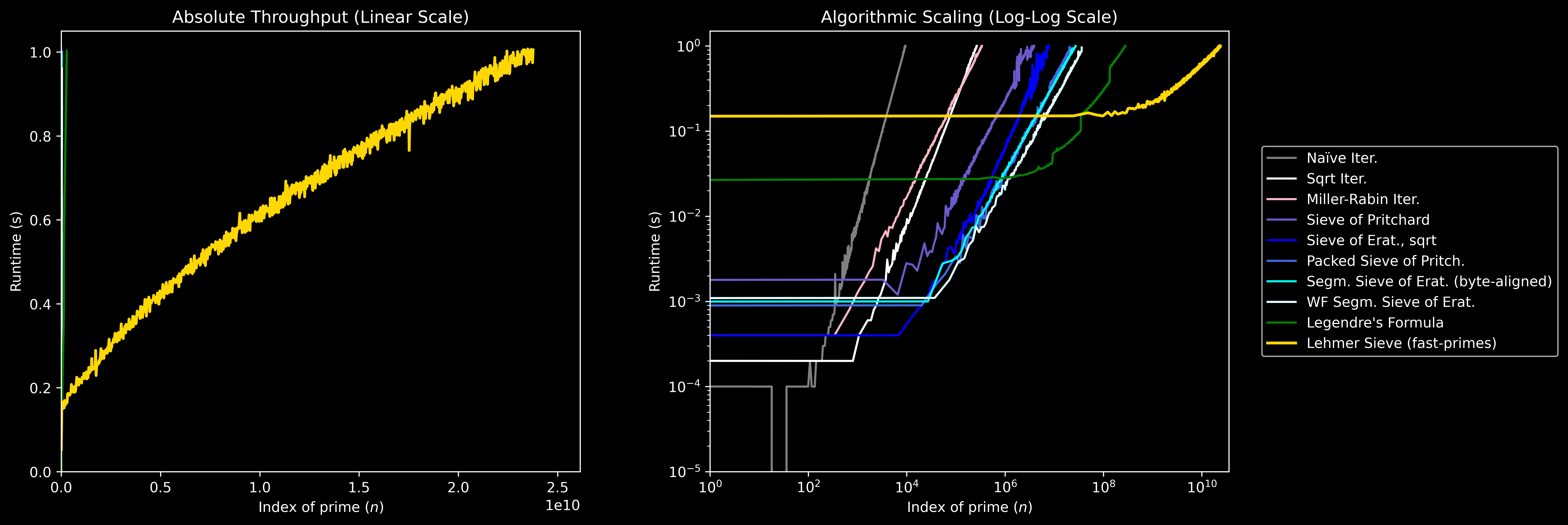
The Linear Scale (Left): On a standard linear axis scaled to the final 23.76 Billion target, the other algorithms are almost crushed against the Y-axis. This is because the traditional sieves and Legendre’s formula hit the 1.0 second mark in the low millions.

The Log-Log Scale (Right): To actually see the mathematical scaling, we use a Log-Log plot, where polynomial time complexities map to straight lines. At the 1.0-second ceiling, the Lehmer curve sits nearly two full orders of magnitude to the right of Legendre’s sieve algorithm.

What the wheel buys — and what it doesn’t

The wheel factorisation in QueenJewels is genuinely elegant. By building on the first 5 primes, the period-2310 wheel visits only the $\phi(2310) = 480$ integers per period that are coprime to $\{2, 3, 5, 7, 11\}$, or about 20.8% of all integers. Every mark in the inner loop lands on a wheel-valid position, and delta encodes the variable gaps so no wasted steps occur.

In fast-primes, the Phase 3 sieve is simpler — a flat byte array, one byte per integer, no wheel. It marks composites with simple stride loops and scans linearly. For a window of ~11 MB, this is fast enough that the simplicity is a feature: the entire sieve fits in L3 cache and the access pattern is perfectly sequential.

The wheel pays for itself in a full-range sieve where you’re visiting every segment from 2 to $p_n$. When you only need to touch an 11 MB window near the answer, the amortised cost of constructing and maintaining the wheel structure outweighs the benefit of visiting fewer positions per segment. The analytic targeting in Phase 1 and 2 already did the heavy lifting.

---

Final Thoughts

The reason this approach is so much faster isn’t a single clever trick — it’s the composition of several ideas that each eliminate a different source of wasted work:

• The Prime Number Theorem tells us roughly where the answer lives.
• The Logarithmic Integral pins that estimate precisely enough to sieve a tiny window.
• Newton-Raphson inverts the li(x) estimate in microseconds.
• Lehmer’s formula counts primes sub-linearly instead of scanning.
• The primorial table makes the $\phi(x, a)$ base case free.
• Fibonacci hashing keeps the memoization table collision-free and cache-friendly.
• Direct syscalls eliminate every layer of runtime overhead.

Each of these is independently interesting. Together they produce something that feels almost unreasonably fast.

The full source — every .ll file, the Makefile, the README and the references — are at github.com/0bVdnt/fast-primes. If you find a bug, have a question about the mathematics, or see a way to push the limit further, I’d genuinely like to hear it.

References: Lehmer (1959), Lagarias–Miller–Odlyzko (1985), Crandall & Pomerance “Prime Numbers: A Computational Perspective” (2005), and SheafificationOfG’s QueenJewels repository for the baseline algorithm implementations and syscall wrappers.